Welcome to the Analytic Tools Documentation!
If you are reading this, you probably got here from GitHub. This is the reference manual detailing the routines and modules of our computational tools for neuroscience package. If you have any questions or comments please do not hesitate to contact .
Note: These pages contain documentation only, to download the code, please refer to the corresponding GitHub repository.
We can only see further by standing on the shoulders of giants - thus, all routines discussed here make heavy use of numerous third party packages. At the very least, NumPy, SciPy and Matplotlib need to be installed on your system in order to use our codes. The following table provides a brief overview of available routines sorted by application area.
| Applications | Routines | Brief Description |
| Network Science | Network Metrics | Computation of simple graph metrics |
| Statistical Dependence Matrices | Calculation of the statistical dependence between sets of time-series | |
| Network Processing | Thresholding, group-averaging and random graph construction | |
| Network Visualization | Illustration of networks in 2D/3D | |
| Miscellaneous | Quality of life improvements for dealing with graphs in Python | |
| Interactive Brain Network Visualization | JavaScript/Plotly Interface | Embedding of networks in three-dimensional brain surfaces |
| Intracranial EEG Data Processing | Read and Convert Raw iEEG Recordings | Pre-processing of intracranial EEG data |
| iEEG Processing Pipeline | Data analysis and assessment | |
| Comparative Statistics | Permutation Testing | Group-level statistical inference |
| General-Purpose Convenience Functions | Array Assessment and Manipulation | Viewing, changing and selecting arrays and their elements |
| File Operations | Inspection, selection and management of files and directories | |
| Neural Population Modeling | Launching a Simulation | Routines to run a simulation with our neural population model |
| Working with the Model | Tools to incorporate coupling matrices and brain parcellations into our model |
Getting Started
The source code of this package is hosted at GitHub. To use the package, create a new directory and either click on the big green download button on the top right of the GitHub page, or open a terminal, go to the newly created directory and type
$ git clone https://github.com/pantaray/Analytic-Tools
Launch Python (we recommend using an iPython shell) and type
>>> from analytical_tools import *
to import the entire collection of modules provided in the package. To import only the network science module, for instance, use
>>> from analytical_tools import nws_tools
Then typing
>>> nws_tools.normalize?
in iPython will display help test for the function normalize() of the network science module nws_tools.py.
Network Science
The Python module nws_tools.py represents a collection of routines for the creation,
processing, analysis and visualization of functional brain networks
(or, in general: weighted, undirected networks).
Network Metrics
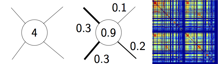
Illustration of three basic graph metrics. Nodal degree quantifies the number of connected edges per node (left), nodal strength reflects the sum of connected link weights (weighted degree) (middle), while connection density denotes the ratio of actual to maximally possible edges in the network (right).
Three basic routines are provided to compute nodal degree and strength as well as connection density
of an undirected graph. Note that similar functions are part of the Brain Connectivity Toolbox
for Python (bctpy). For convenience the routines are included in
nws_tools anyway in case bctpy is not available.
Click on a specific routine to see more details.
degrees_und(CIJ) |
Compute nodal degrees in an undirected graph |
strengths_und(CIJ) |
Compute nodal strengths in an undirected graph |
density_und(CIJ) |
Compute the connection density of an undirected graph |
Statistical Dependence Matrices
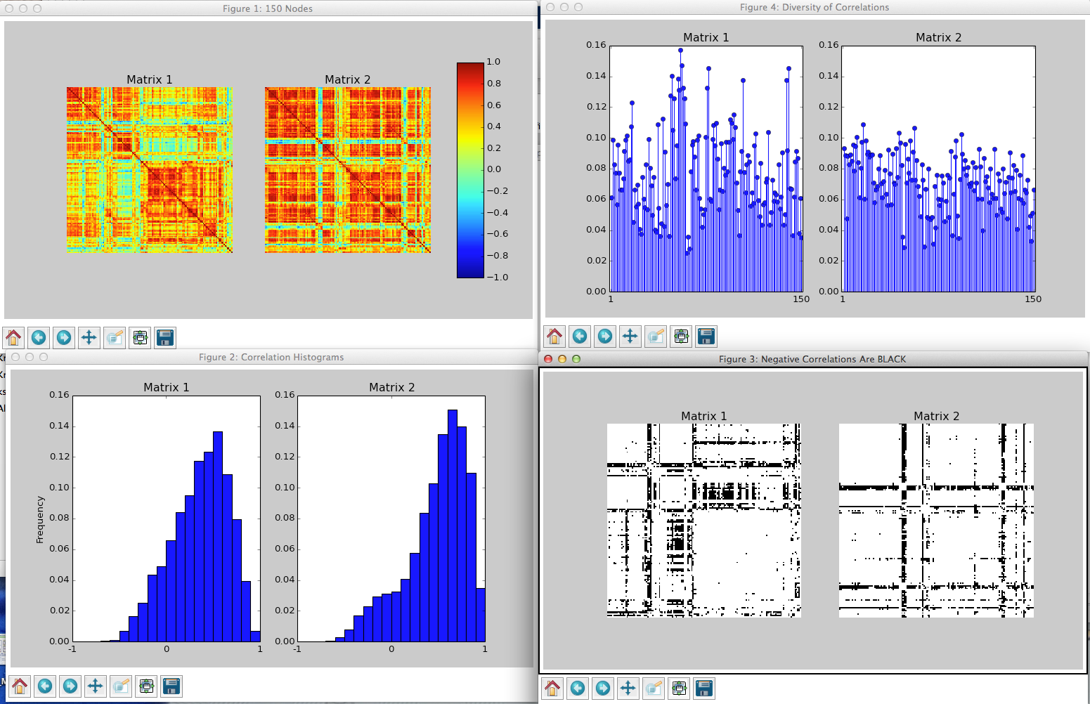
Exemplary output of the routine corrcheck() showing two Pearson correlation matrices.
The routines below may be used to generate, process and visually inspect functional connection matrices based on different notions of statistical dependence.
get_corr(txtpath[, corrtype, sublist]) |
Compute pair-wise statistical dependence of time-series |
mutual_info(tsdata[, n_bins, normalized, ...]) |
Calculate a (normalized) mutual information matrix at zero lag |
corrcheck(*args, **kwargs) |
Sanity checks for statistical dependence matrices |
rm_negatives(corrs) |
Remove negative entries from connection matrices |
rm_selfies(conns) |
Remove self-connections from connection matrices |
issym(A[, tol]) |
Check for symmetry of a 2d NumPy array |
Network Processing
A collection of routines providing means to average and threshold networks as well as to generate a number of null model graphs.
get_meannw(nws[, percval]) |
Helper function to compute group-averaged networks |
thresh_nws(nws[, userdens, percval, ...]) |
Threshold networks based on connection density |
generate_randnws(nw, M[, method, rwr, rwr_max]) |
Generate random networks given a(n) (un)signed (un)weighted (un)directed input network |
Network Visualization
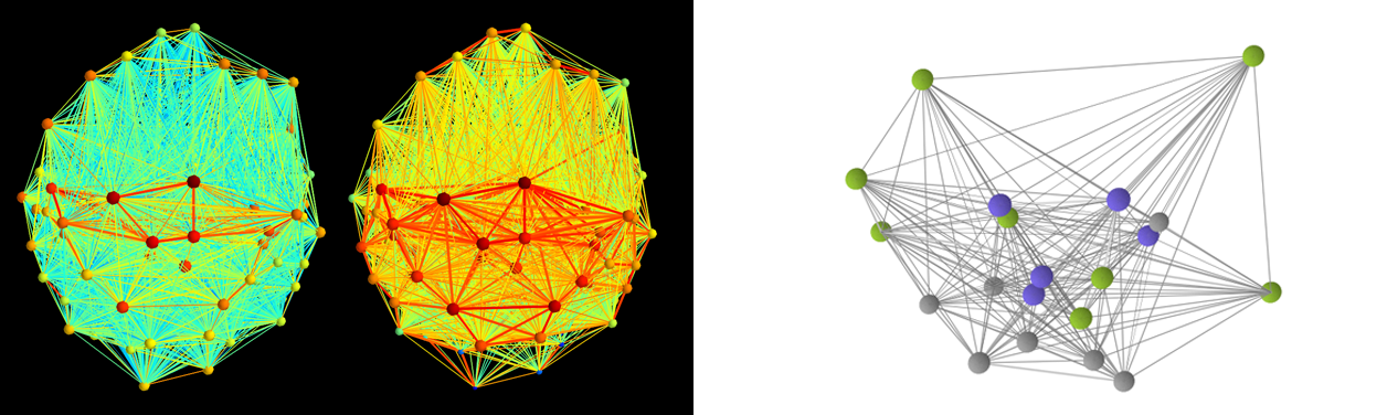
Two functional brain networks generated using shownet() (left)
and a graph rendered with show_nw() (right).
The following routines may be useful for rendering networks using either Mayavi or Matplotlib.
shownet(A, coords[, colorvec, sizevec, ...]) |
Plots a network in 3D using Mayavi |
show_nw(A, coords[, colorvec, sizevec, ...]) |
Matplotlib-based plotting routine for networks |
csv2dict(csvfile) |
Reads 3D nodal coordinates of from a csv file into a Python dictionary |
Miscellaneous
Routines that may come in handy when working with networks and large data files.
normalize(arr[, vmin, vmax]) |
Re-scales a NumPy ndarray |
nw_zip(ntw) |
Convert the upper triangular portion of a real symmetric matrix to a vector and vice versa |
hdfburp(f) |
Pump out everything stored in a HDF5 container |
printdata(data, leadrow, leadcol[, fname]) |
Pretty-print/-save array-like data |
img2vid(imgpth, imgfmt, outfile, fps[, ...]) |
Convert a sequence of image files to a video using ffmpeg |
Interactive Brain Network Visualization
The module plotly_tools.py can be used to automate common laborious tasks when
creating interactive visualizations of networks embedded in three-dimensional renderings
of brain surfaces using Plotly.
JavaScript/Plotly Interface
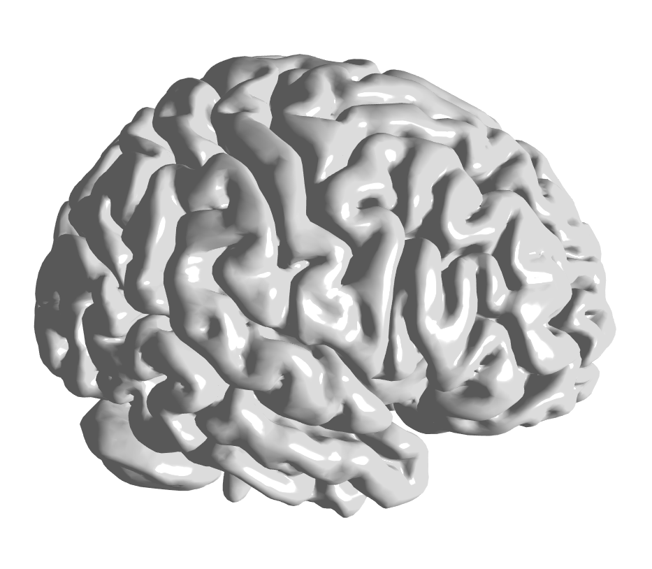
Exemplary rendering of the brain surface BrainMesh_Ch2withCerebellum
provided in the HDF5 container brainsurf.h5 located in the brainsurf
sub-directory of the package.
These functions might simplify the creation of HTML files with Plotly.
cmap_plt2js(cmap[, cmin, cmax, Ncols]) |
Converts Matplotlib colormaps to JavaScript color-scales |
make_brainsurf(surfname[, orientation, ...]) |
Create Plotly graph objects to render brain surfaces |
Intracranial EEG Data Processing
The module eeg_tools.py contains a number of routines that we developed for our research
in human intracranial electrophysiology.
Note: These codes are work in progress designed with our specific workflow requirements in mind. If you need a widely tested, full-fledged general purpose toolbox to analyze electrophysiological data, consider using FieldTrip.
Read and Convert Raw iEEG Recordings
Two routines to (1) read raw iEEG recordings from *.eeg/*.21E files and store the data in more accessible HDF5 containers and (2) subsequently access the generated data-sets.
read_eeg(eegpath, outfile[, electrodelist, ...]) |
Read raw EEG data from binary *.EEG/*.eeg and *.21E files |
load_data(h5file[, nodes]) |
Load data from HDF5 container generated with read_eeg |
iEEG Processing Pipeline
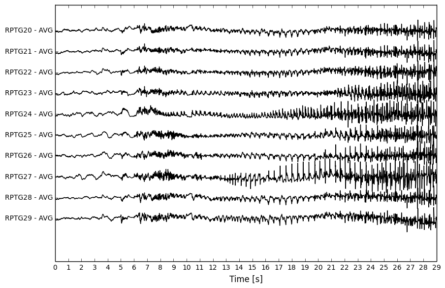
Pre-processed 10-channel iEEG segment.
Functions to perform routine tasks on (pre-processed) iEEG recordings.
bandpass_filter(signal, locut, hicut, srate) |
Band-/Low-/High-pass filter a 1D/2D input signal |
MA(signal, window_size[, past]) |
Smooth 1d/2darray using a moving average filter along one axis |
time2ind(h5file, t_start, t_end) |
Convert human readable 24hr times to indices used in given iEEG file container |
Comparative Statistics
The module stats_tools.py may be used to assess the statistical significance of group-level differences
in two-sample problems.
Permutation Testing
The core of this module is a wrapper that invokes third party packages to perform group-level statistical inference. Thus, depending on the use-case the Python packages MNE, Pandas, rpy2, as well as the external software environment R including the R-library flip are required.
perm_test(X, Y[, paired, useR, nperms, ...]) |
Perform permutation tests for paired/unpaired uni-/multi-variate two-sample problems |
printstats(variables, pvals, group1, group2) |
Pretty-print previously computed statistical results |
General-Purpose Convenience Functions
The module recipes.py represents a collection of tools to perform a variety of common tasks one tends to run into
when working with NumPy arrays and large file cohorts in Python.
Array Assessment and Manipulation
Most of these routines encapsulate code segments that repeatedly proved to be useful when performing seemingly “straight-forward” operations on NumPy arrays.
natural_sort(lst) |
Sort a list/NumPy 1darray in a “natural” way |
regexfind(arr, expr) |
Find regular expression in a NumPy array |
query_yes_no(question[, default]) |
Ask a yes/no question via raw_input() and return the answer. |
File Operations
A few file-system I/O functions that might make everyday read/write operations a little less tedious.
myglob(flpath, spattern) |
Return a glob-like list of paths matching a regular expression |
get_numlines(fname) |
Get number of lines of an text file |
moveit(fname) |
Check if a file/directory exists, if yes, rename it |
Neural Population Modeling
In contrast to the tools discussed above, the source code of the Python/Cython implementation of our
neural population model is not encapsulated in a single module. Thus, more than one *.py file
is required to perform a neural simulation.
More specifically, the code-base of the model makes extensive use of Cython, an optimizing static compiler providing C extensions for Python. Thus, unlike pure Python modules, to run a simulation the model sources have to be built first. To do that, Cython needs to be installed (please refer to these guides for installation instructions). Further, to accelerate matrix-vector multiplications, our code relies on CBLAS routines and thus requires a full installation of the CBLAS library (including header files). Once these dependencies are installed, open a terminal in the directory you downloaded the Analytic Tools package to and type
$ make all
This will first convert the Cython module the_model.pyx to a C source code file the_model.c,
which will be subsequently compiled and linked based on the options specified in setup.py to generate
a shared object called the_model.so. Now, the model is ready to perform simulations.
The Simulation Module
To streamline the generation of whole brain simulations, a Python module called sim_tools.py
is provided that acts as a launch manager and is intended as “Pythonic” layer between the user and
the model’s C-extension. Note that the use of sim_tools.py is encouraged but not required - feel free
to write your own management routines by looking at the source code of the function run_model()
in sim_tools.py.
Launching a Simulation
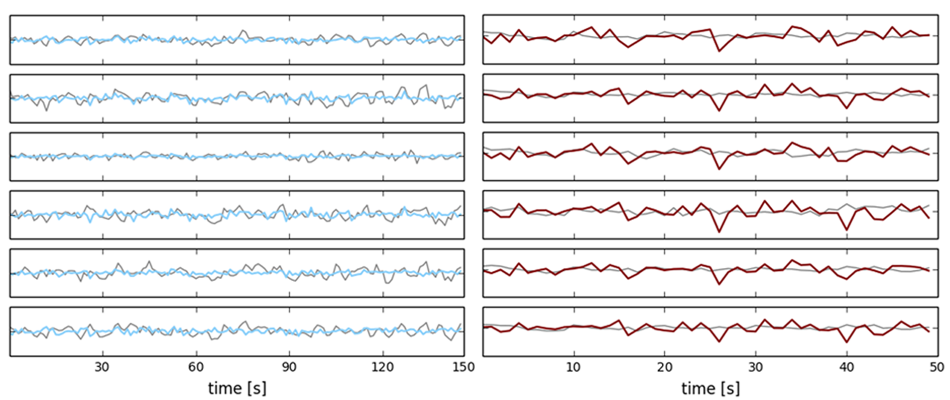
Exemplary simulations compared to empirical BOLD signals.
The following routines in sim_tools.py are intended to run simulations and plot the corresponding
results.
run_model(V0, Z0, DA0, task, outfile[, ...]) |
Run a simulation using the neural population model |
make_bold(fname[, stim_onset]) |
Convert raw model output to BOLD signal |
plot_sim(fname[, names, raw, bold, figname]) |
Plot a simulation generated by run_model |
Working with the Model
The functions below are not essential for using the model, but might come in handy nonetheless.
show_params(fname) |
Pretty-print all parameters used in a simulation |
make_D(target, source, names[, values]) |
Create matrix of afferent/efferent dopamine regions in the model |